Simulating AIA 171 Emission from a Bundle of Strands

This example shows how to model AIA emission from a bundle of semi-circular strands for two different viewpoints.

import matplotlib.pyplot as plt
import astropy.time
import astropy.units as u
from astropy.visualization import quantity_support
from astropy.coordinates import SkyCoord
from sunpy.map import pixelate_coord_path, sample_at_coords

import synthesizAR
from synthesizAR.instruments import InstrumentSDOAIA
from synthesizAR.interfaces import RTVInterface
from synthesizAR.models import semi_circular_bundle
# sphinx_gallery_thumbnail_number = -1

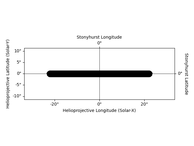
First, we calculate a list of coordinates comprising a semi-circular bundle of strands. The bundle has a length of 50 Mm and a cross-sectional radius of 1 Mm and a total of 500 strands. The strands are uniformly distributed over the bundle.

obstime = astropy.time.Time.now()
pos = SkyCoord(
    lon=0*u.deg, lat=0*u.deg, radius=1*u.AU, obstime=obstime, frame='heliographic_stonyhurst')
bundle_coords = semi_circular_bundle(50 * u.Mm, 1*u.Mm, 500, observer=pos)

As in other examples, we then use the coordinates of our strands to construct the Skeleton object.

strands = [synthesizAR.Loop(f'strand{i}', c) for i, c in enumerate(bundle_coords)]
bundle = synthesizAR.Skeleton(strands)
bundle.peek(observer=pos)

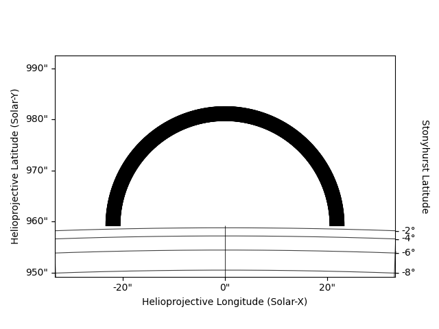
We can also look at our bundle of strands from the side to confirm it has the desired geometry.

side_on_view = SkyCoord(lon=0*u.deg, lat=-90*u.deg, radius=1*u.AU, frame=pos.frame)
bundle.peek(observer=side_on_view, grid_kwargs={'grid_spacing': 2*u.deg})

We will again use a simple RTV loop model to compute the thermal structure of each strand. This assigns a single temperature density to the entire loop based on the loop length and the specified heating rate.

rtv = RTVInterface(heating_rate=1e-4*u.Unit('erg cm-3 s-1'))
bundle.load_loop_simulations(rtv)

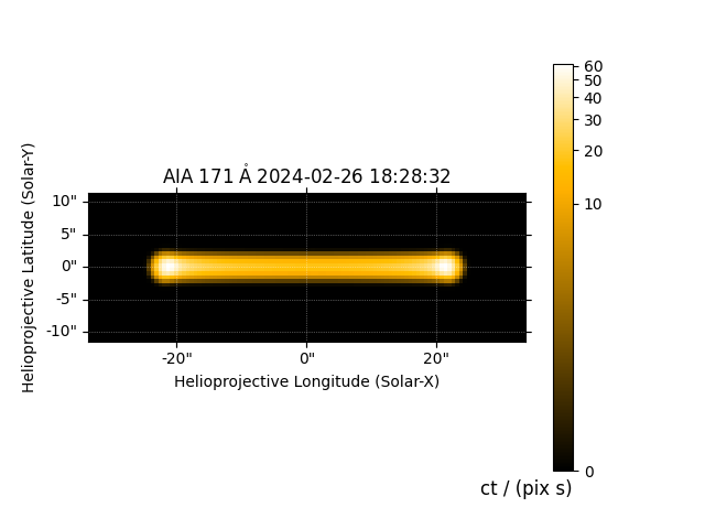
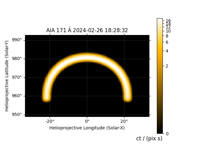
We can then compute the emission as observed by the 171 channel of AIA as viewed from an observer at 1 AU directly above the loop.

aia = InstrumentSDOAIA([0, 1]*u.s, pos, pad_fov=(10, 10)*u.arcsec)
maps = aia.observe(bundle, channels=aia.channels[2:3])
m_171 = maps['171'][0]
m_171.peek()

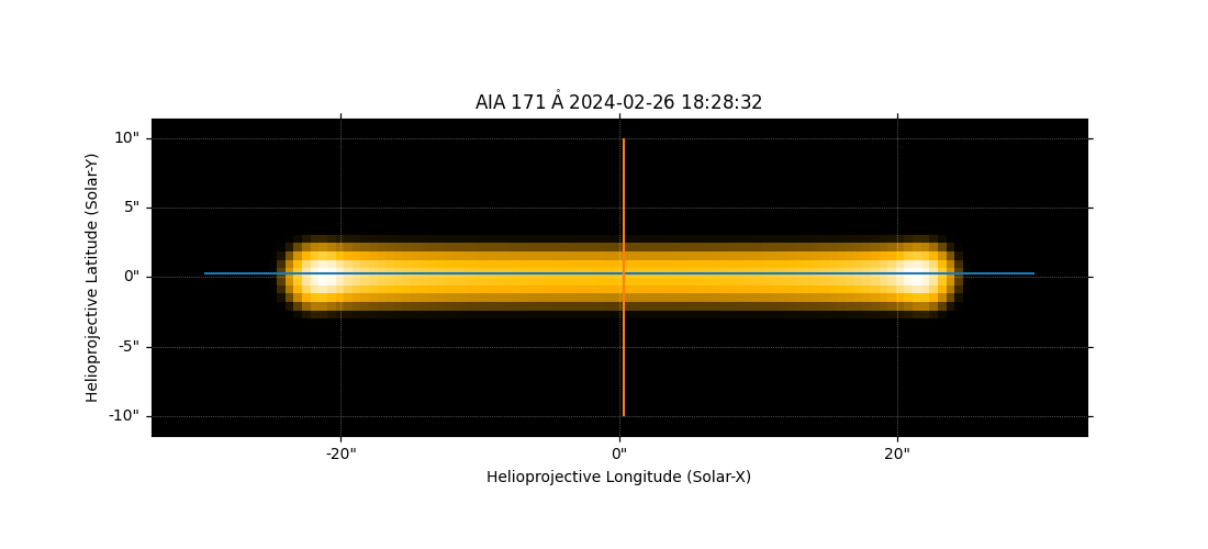
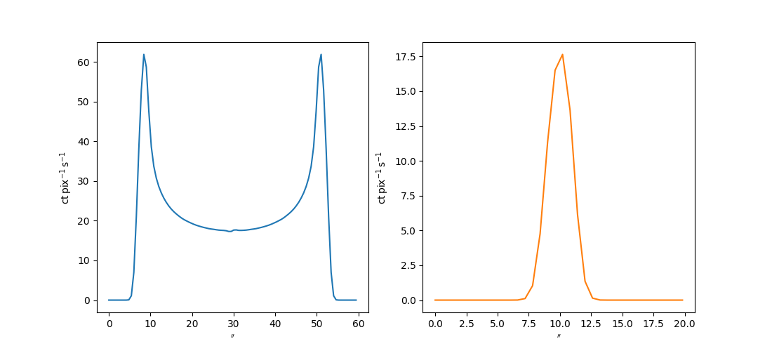
Additionally, we can look at intensity profiles along and across the loop axis using sunpy.map.pixelate_coord_path and sunpy.map.sample_at_coords.

coord_axis = SkyCoord(Tx=[-30, 30]*u.arcsec, Ty=0*u.arcsec,
                      frame=m_171.coordinate_frame)
coord_axis = pixelate_coord_path(m_171, coord_axis)
profile_axis = sample_at_coords(m_171, coord_axis)
coord_xs = SkyCoord(Tx=0*u.arcsec, Ty=[-10, 10]*u.arcsec,
                    frame=m_171.coordinate_frame)
coord_xs = pixelate_coord_path(m_171, coord_xs)
profile_xs = sample_at_coords(m_171, coord_xs)

Note that the intensity is highest at the footpoints because we are integrating through the most amount of plasma. Additionally, note that the cross-sectional profile has a width consistent with the spatial radius we specified when constructing our bundle of strands.

fig = plt.figure(figsize=(11, 5))
ax = fig.add_subplot(111, projection=m_171)
m_171.plot(axes=ax)
ax.plot_coord(coord_axis)
ax.plot_coord(coord_xs)
with quantity_support():
    plt.figure(figsize=(11, 5))
    plt.subplot(121)
    plt.plot(coord_axis.separation(coord_axis[0]).to('arcsec'), profile_axis, color='C0')
    plt.subplot(122)
    plt.plot(coord_xs.separation(coord_xs[0]).to('arcsec'), profile_xs, color='C1')

• 
• 

Finally, we can also compute the AIA 171 intensity as viewed from the side in order to see the semi-circular geometry of the loop bundle.

aia = InstrumentSDOAIA([0, 1]*u.s, side_on_view, pad_fov=(10, 10)*u.arcsec)
maps = aia.observe(bundle, channels=aia.channels[2:3])
maps['171'][0].peek()