Simulating Time-dependent Emission from Impulsively Heated Loops with EBTEL

This example demonstrates how to model the resulting AIA emission from an arcade of loops heated impulsively and modeled using the ebtelplusplus code.

import astropy.time
import astropy.units as u
import matplotlib.pyplot as plt
import numpy as np
import sunpy.map

from astropy.coordinates import SkyCoord
from astropy.visualization import AsinhStretch, ImageNormalize, quantity_support
from sunpy.coordinates import get_horizons_coord

import synthesizAR

from synthesizAR.instruments.sdo import InstrumentSDOAIA
from synthesizAR.interfaces.ebtel import EbtelInterface
from synthesizAR.interfaces.ebtel.heating_models import PowerLawNanoflareTrain
from synthesizAR.models import semi_circular_arcade

# sphinx_gallery_thumbnail_number = -1

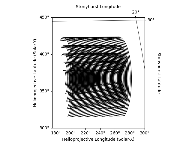
First, set up the coordinates for the arcade. The structure we will model is an arcade of longer overlying loops with an arcade of successively shorter loops underneath.

obstime = astropy.time.Time('2022-11-14T22:00:00')
pos = SkyCoord(lon=15*u.deg,
               lat=25*u.deg,
               radius=1*u.AU,
               obstime=obstime,
               frame='heliographic_stonyhurst')
arcade_coords = []
delta_s = 0.3 * u.Mm
for l in np.arange(25,150,25)*u.Mm:
    n_points = int(np.ceil((l/delta_s).decompose()))
    arcade_coords += semi_circular_arcade(l, 5*u.deg, 50, pos, n_points=n_points)

Next, build a Skeleton from the coordinates of the strands in our arcade.

strands = [synthesizAR.Strand(f'strand{i}', c) for i, c in enumerate(arcade_coords)]
arcade = synthesizAR.Skeleton(strands)

We can visualize what this structure would look like as observed from the Solar Dynamics Observatory.

sdo_observer = get_horizons_coord('SDO', time=obstime)
arcade.peek(observer=sdo_observer,
            axes_limits=[(175, 300)*u.arcsec, (300, 450)*u.arcsec])

INFO: Obtained JPL HORIZONS location for Solar Dynamics Observatory (spacecraft) (-136395) [sunpy.coordinates.ephemeris]

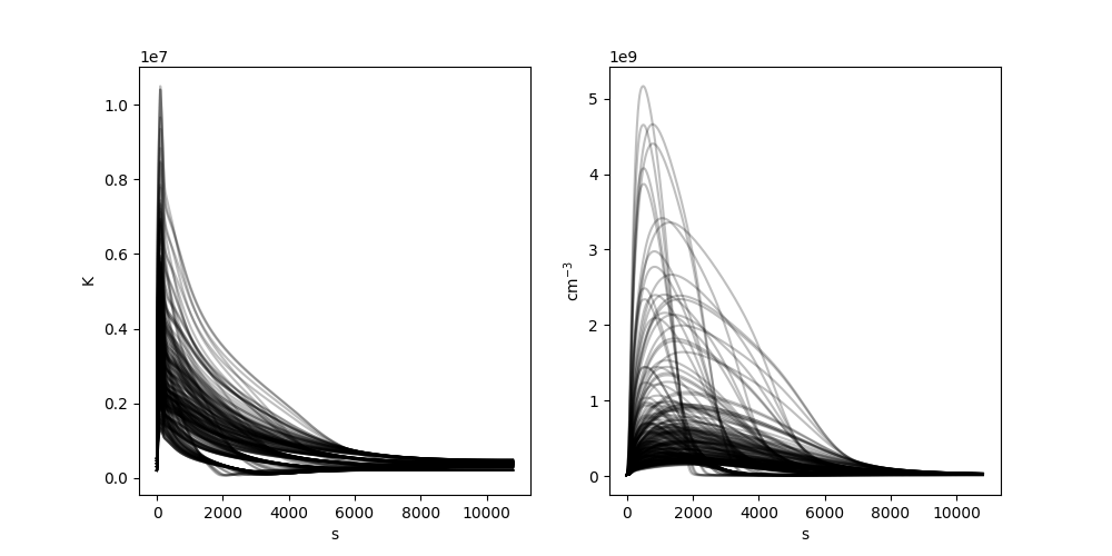
Next, we will model the hydrodynamic response to an impulsive heating event on each strand using the ebtelplusplus code. We will simulate a total of 3 h of simulation time where each loop is heated by a single event with an energy chosen from a powerlaw distribution.

event_model = PowerLawNanoflareTrain(
    [0,200]*u.s, 200*u.s, 0*u.s, [1e-3,1e-1]*u.Unit('erg cm-3 s-1'), -1.5
)
ebtel = EbtelInterface(3*u.h, event_builder=event_model)

To attach the results of our loop simulation to each strand, we pass the interface to the geometric model of our arcade we built above.

arcade.load_loop_simulations(ebtel)

We can then visualize the temperature and density evolution of each strand as a function of time. Note that because EBTEL is a spatially-averaged model, it is assumed that eadch point along the strand has the same temperature and density.

with quantity_support():
    fig = plt.figure(figsize=(10,5))
    ax1 = fig.add_subplot(121)
    ax2 = fig.add_subplot(122)
    for s in arcade.strands:
        ax1.plot(s.time, s.electron_temperature[:,0], color='k', alpha=0.25)
        ax2.plot(s.time, s.density[:,0], color='k', alpha=0.25)

The last step is to use the temperature and density along each strand to compute the emission as observed by the AIA instrument. We’ll model the emission from 500 s to 6000 s at a cadence of 50 s for the 193 Å channel.

aia = InstrumentSDOAIA(np.arange(500,6e3,50)*u.s,
                       sdo_observer,
                       pad_fov=(40, 40)*u.pixel)
maps = aia.observe(arcade, channels=aia.channels[3:4])

INFO: Apparent body location accounts for 493.59 seconds of light travel time [sunpy.coordinates.ephemeris]

We can easily visualize this time-dependent emission using a MapSequence.

mseq = sunpy.map.Map(maps['193'], sequence=True)
fig = plt.figure()
ax = fig.add_subplot(projection=mseq[0])
ani = mseq.plot(axes=ax, norm=ImageNormalize(vmin=0, vmax=5, stretch=AsinhStretch()))

plt.show()

Once Loop Reflect