Modeling an Arcade of Loops with the RTV Scaling Laws

This example shows how to model AIA emission from an arcade of semi-circular loops who’s thermal structure is modeled using the RTV scaling laws.

import astropy.units as u
import astropy.time
from astropy.coordinates import SkyCoord
from sunpy.coordinates import get_earth

import synthesizAR
from synthesizAR.models import semi_circular_arcade
from synthesizAR.interfaces import RTVInterface
from synthesizAR.instruments import InstrumentSDOAIA

First, set up the coordinates for loops in the arcade.

obstime = astropy.time.Time('2022-11-14T22:00:00')
pos = SkyCoord(lon=15*u.deg, lat=25*u.deg, radius=1*u.AU, obstime=obstime, frame='heliographic_stonyhurst')
arcade_coords = semi_circular_arcade(80*u.Mm, 5*u.deg, 50, pos, inclination=10*u.deg)

Next, assemble the arcade.

strands = [synthesizAR.Loop(f'strand{i}', c) for i, c in enumerate(arcade_coords)]
arcade = synthesizAR.Skeleton(strands)

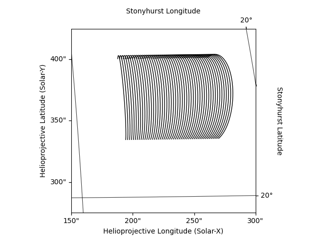
We can make a quick plot of what these coordinates would look like as viewed from Earth.

earth_observer = get_earth(obstime)
arcade.peek(observer=earth_observer,
            axes_limits=[(150, 300)*u.arcsec, (275, 425)*u.arcsec])

Next, model the thermal structure of each loop using the RTV scaling laws.

rtv = RTVInterface(heating_rate=1e-6*u.Unit('erg cm-3 s-1'))
arcade.load_loop_simulations(rtv)

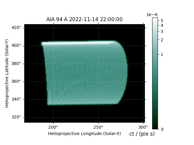
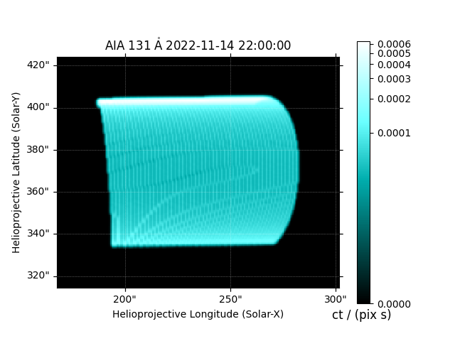
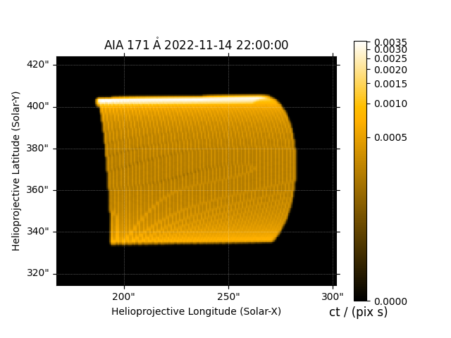
Finally, compute the LOS integrated AIA emission.

aia = InstrumentSDOAIA([0, 1]*u.s, earth_observer, pad_fov=(20, 20)*u.arcsec)
maps = aia.observe(arcade)

Files Downloaded:   0%|          | 0/1 [00:00<?, ?file/s]

aiapy.aia_V8_all_fullinst.genx:   0%|          | 0.00/5.43M [00:00<?, ?B/s]

aiapy.aia_V8_all_fullinst.genx:  11%|█         | 593k/5.43M [00:00<00:00, 5.93MB/s]

aiapy.aia_V8_all_fullinst.genx:  69%|██████▉   | 3.73M/5.43M [00:00<00:00, 20.8MB/s]


Files Downloaded: 100%|██████████| 1/1 [00:00<00:00,  3.01file/s]
Files Downloaded: 100%|██████████| 1/1 [00:00<00:00,  3.00file/s]

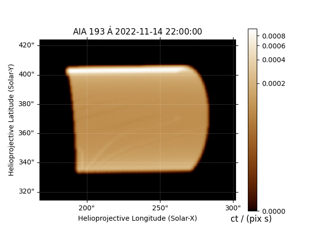
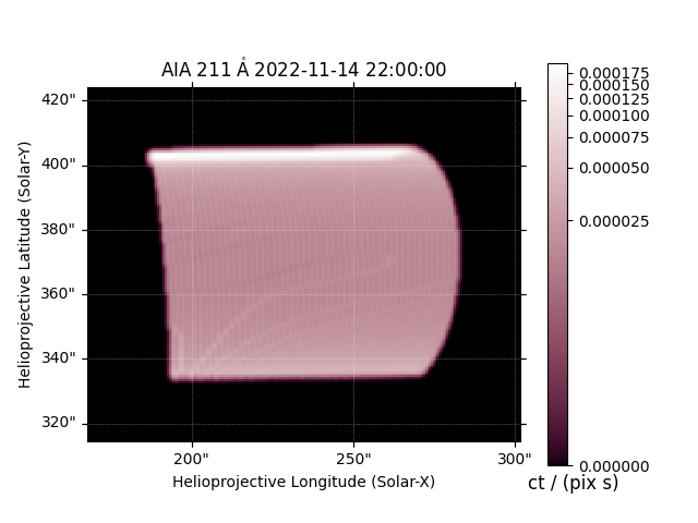
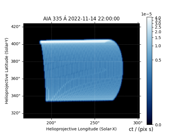
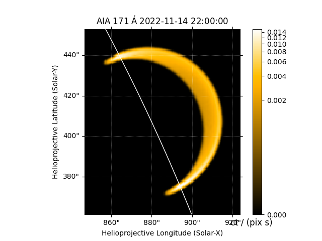
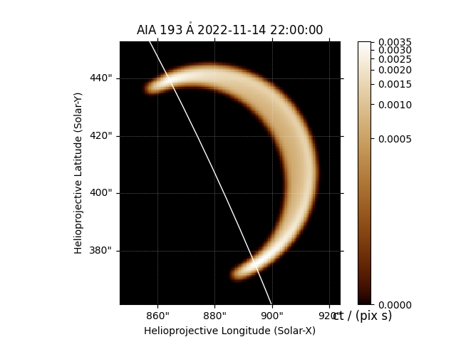
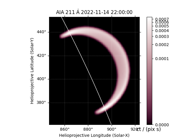
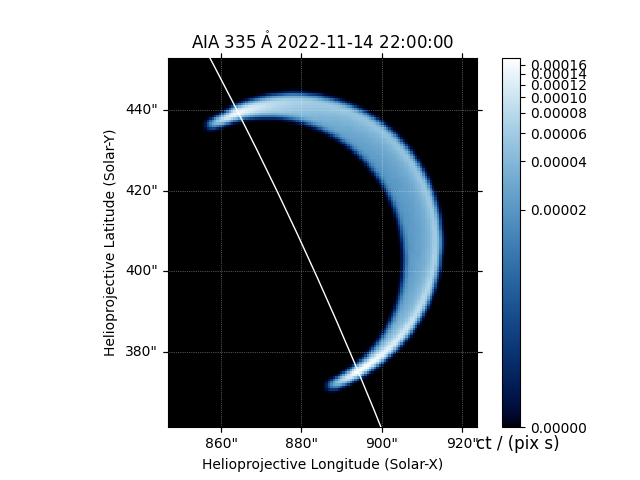
We can make a quick plot of what each EUV channel of AIA would look like.

for k in maps:
    maps[k][0].peek()

• 
• 
• 
• 
• 
• 

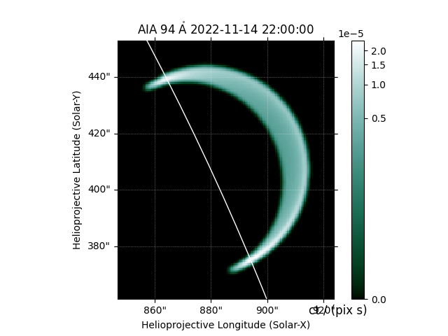
We can easily adjust the viewing angle to integrate the emission along a different LOS.

off_limb_observer = SkyCoord(
    lon=-70*u.deg, lat=earth_observer.lat, radius=earth_observer.radius, frame=earth_observer.frame)
aia = InstrumentSDOAIA([0, 1]*u.s, off_limb_observer, pad_fov=(10, 10)*u.arcsec,)
maps = aia.observe(arcade)
for k in maps:
    maps[k][0].peek(draw_limb=True)

• 
• 
• 
• 
• 
•