Modeling Intensities from Multiple Instruments

This example shows how to compute the synthetic intensities from three different observatories: AIA, XRT, and EUVI. It also demonstrates how to define a custom instrument class.

import astropy.units as u
import matplotlib.pyplot as plt
import numpy as np

from astropy.coordinates import SkyCoord
from astropy.visualization import quantity_support
from sunpy.coordinates import (
    get_earth,
    get_horizons_coord,
    HeliographicStonyhurst,
    Helioprojective,
)

import synthesizAR

from synthesizAR.instruments.hinode import InstrumentHinodeXRT
from synthesizAR.instruments.sdo import InstrumentSDOAIA
from synthesizAR.interfaces import MartensInterface
from synthesizAR.models import semi_circular_arcade

# sphinx_gallery_thumbnail_number = -1

First, we’ll set up the geometry for the active region that we are modeling. We’ll use a simple arcade of semi-circular loops all with a length of 150 Mm.

obstime = '2021-10-28T15:00:00'
loc = SkyCoord(HeliographicStonyhurst(lon=0*u.deg,lat=-30*u.deg, radius=1*u.R_sun, obstime=obstime))
arcade = semi_circular_arcade(150*u.Mm, 10*u.deg, 50, loc, gamma=90*u.deg, n_points=5000)
skeleton = synthesizAR.Skeleton([synthesizAR.Strand(f'{i}', c) for i,c in enumerate(arcade)])

We’ll select a few different observer locations for SDO and STERO-A and use sunpy.coordinates.get_horizons_coord to get these locations from the JPL Horizons service. We’ll approximate the location of Hinode as Earth since its location is not available through JPL Horizons.

sdo = get_horizons_coord('SDO', time=obstime)
stereo_a = get_horizons_coord('STEREO-A', time=obstime)
hinode = get_earth(time=obstime)

INFO: Obtained JPL HORIZONS location for Solar Dynamics Observatory (spacecraft) (-136395) [sunpy.coordinates.ephemeris]
INFO: Obtained JPL HORIZONS location for STEREO-A (spacecraft) (-234)    [sunpy.coordinates.ephemeris]

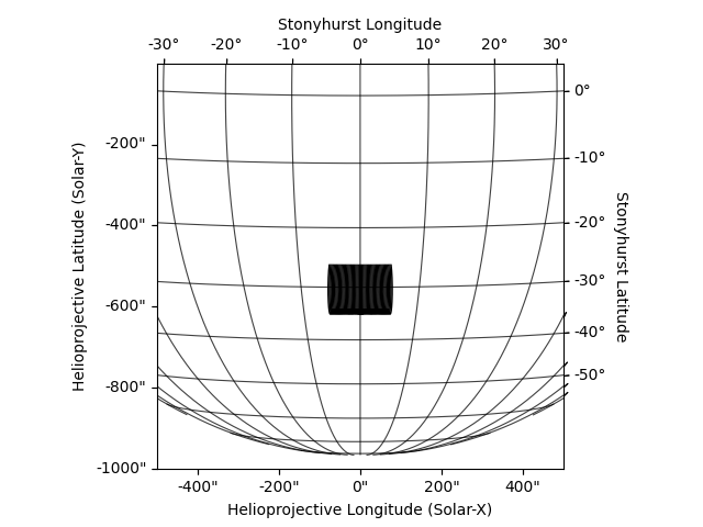
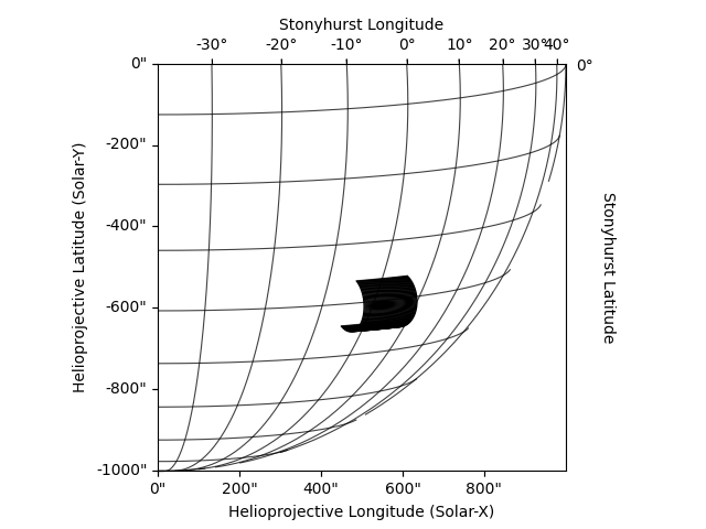
We can quickly peek at what the structure of our active region looks like from the viewpoints of SDO and STEREO-A.

skeleton.peek(observer=sdo, axes_limits=[(-500,500)*u.arcsec, (-1000,0)*u.arcsec])
skeleton.peek(observer=stereo_a, axes_limits=[(0,1000)*u.arcsec, (-1000,0)*u.arcsec])

• 
• 

Next, we want to calculate some sort of thermodynamic model for each one of these strands. We’ll use the MartensScalingLaws model with the heating rate chosen from a uniform distribution.

class MartensRandom(MartensInterface):

    def get_heating_constant(self, loop):
        h_a = 1e-5 * u.Unit('erg cm-3 s-1')
        h_b = 100*h_a
        return h_a + np.random.random_sample()*(h_b - h_a)

martens = MartensRandom(None)
skeleton.load_loop_simulations(martens)

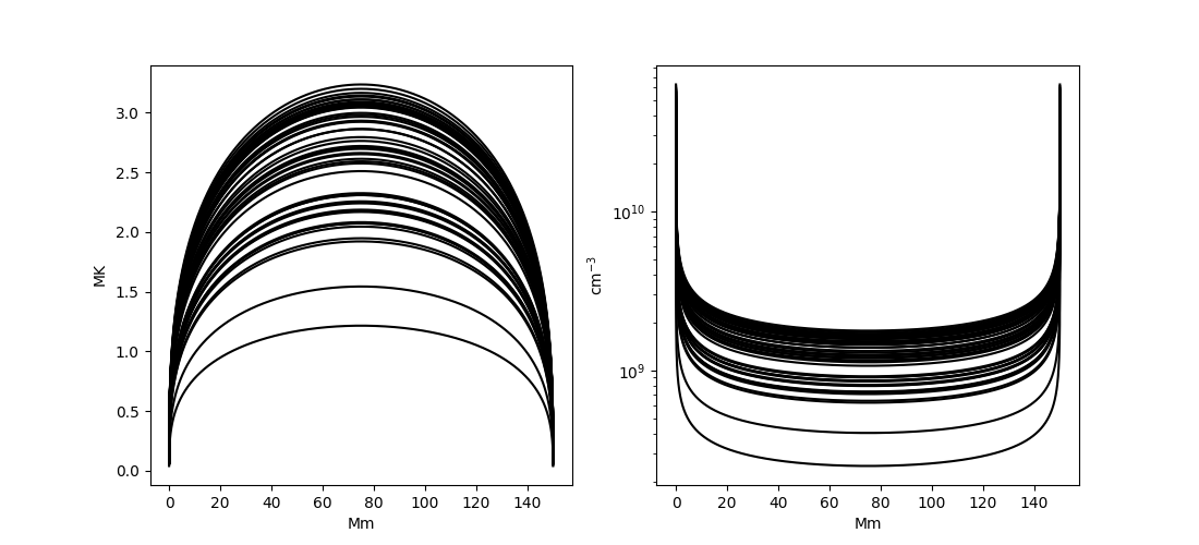
We can visualize the electron temperature and density profiles for each loop.

with quantity_support():
    plt.figure(figsize=(11, 5))
    ax1 = plt.subplot(121)
    for l in skeleton.strands:
        plt.plot(l.field_aligned_coordinate_center.to('Mm'), l.electron_temperature[0].to('MK'), color='k')
    plt.subplot(122)
    for l in skeleton.strands:
        plt.plot(l.field_aligned_coordinate_center.to('Mm'), l.density[0], color='k')
    plt.yscale('log')

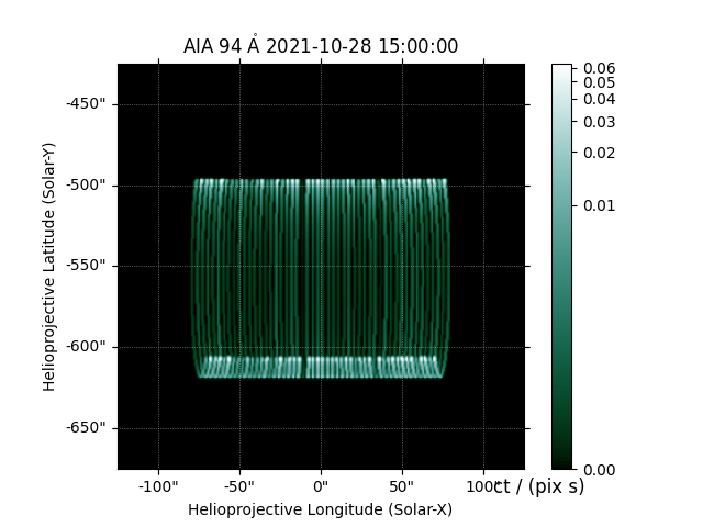
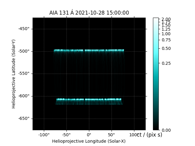
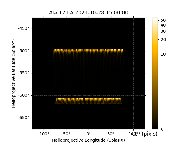
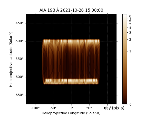
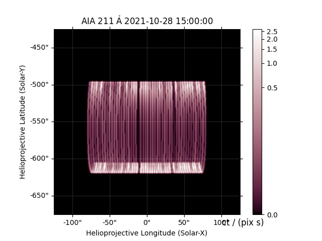
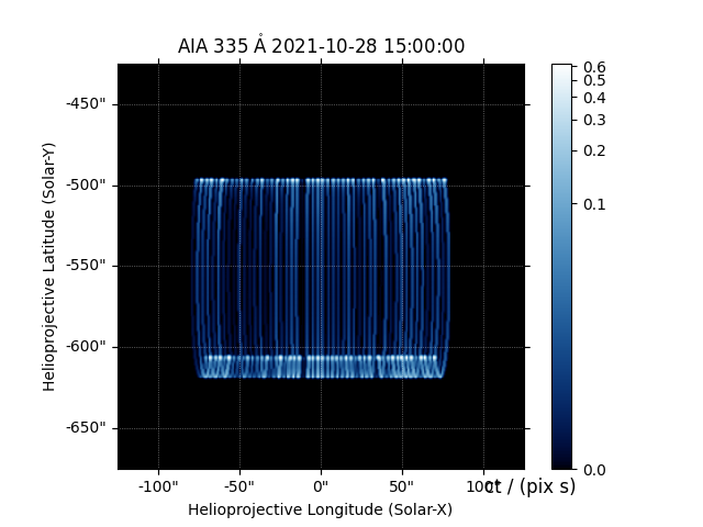
Let’s compute the emission that would be observed from these loops with this particular model for the temperature and density. First, we’ll compute the emission as observed in all channels of AIA. We’ll select a field of view by specifying the center of the field of view as well as the width and height.

center = SkyCoord(Tx=0*u.arcsec, Ty=-550*u.arcsec, frame=Helioprojective(observer=sdo, obstime=sdo.obstime))
fov_width = (250,250)*u.arcsec
aia = InstrumentSDOAIA([0]*u.s, sdo, fov_center=center, fov_width=fov_width)
aia_images = aia.observe(skeleton)
for k in aia_images:
    aia_images[k][0].peek()

• 
• 
• 
• 
• 
• 

INFO: Apparent body location accounts for 495.70 seconds of light travel time [sunpy.coordinates.ephemeris]

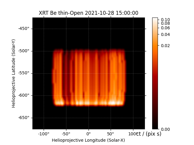
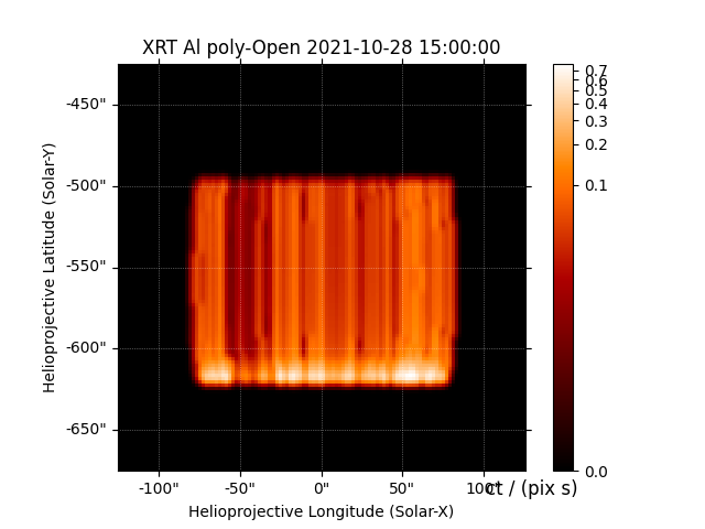
We can carry out this same procedure for Hinode XRT for the same field of view. We’ll look just at the Be-thin and Al-poly channels.

xrt = InstrumentHinodeXRT([0]*u.s, hinode, ['Be-thin', 'Al-poly'],
                          fov_center=center, fov_width=fov_width)
xrt_images = xrt.observe(skeleton)
for k in xrt_images:
    xrt_images[k][0].peek()

• 
• 

INFO: Apparent body location accounts for 495.76 seconds of light travel time [sunpy.coordinates.ephemeris]

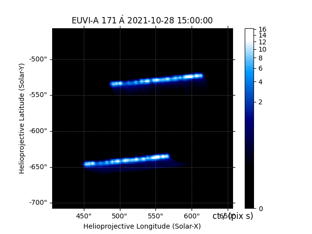
Lastly, we want to compute the emission as observed by EUVI on STEREO-A. Currently, synthesizAR.instruments does not contain an EUVI instrument class. However, we can easily define our own as follows. Note that here, for simplicity, we are using the 171 Å temperature response function for AIA as a proxy for the temperature response of the 171 Å channel on EUVI.

class InstrumentSTEREOEUVI(InstrumentSDOAIA):
    name = 'STEREO_EUVI'

    def __init__(self, *args, **kwargs):
        super().__init__(
            *args,
            plate_scale=u.Quantity([1.58777404, 1.58777404], 'arcsec / pixel'),
            cadence=1*u.h,
            **kwargs,
        )

    @property
    def observatory(self):
        return 'STEREO A'

    @property
    def telescope(self):
        return 'STEREO'

    @property
    def detector(self):
        return 'EUVI'

    def get_instrument_name(self, *args):
        return 'SECCHI'

We can then use our custom instrument class in the exact same way as our predefined classes to model the emission from EUVI. Note that we’ll only do this for the 171 Å channel.

euvi = InstrumentSTEREOEUVI([0]*u.s, stereo_a, fov_center=center, fov_width=fov_width)
euvi_images = euvi.observe(skeleton, channels=euvi.channels[2:3])
euvi_images['171'][0].peek()

INFO: Apparent body location accounts for 478.19 seconds of light travel time [sunpy.coordinates.ephemeris]